How to Find What’s Driving BigQuery Bytes Billed

Recently, I reduced BigQuery cost significantly by changing how we maintained a token index table used for keyword search.

The original design updated the index during ingestion. Each small OCR batch triggered a MERGE into a chunk_terms table. That looked incremental, but it turned out to be expensive because BigQuery still needed to scan the target table on every MERGE to check for matches.

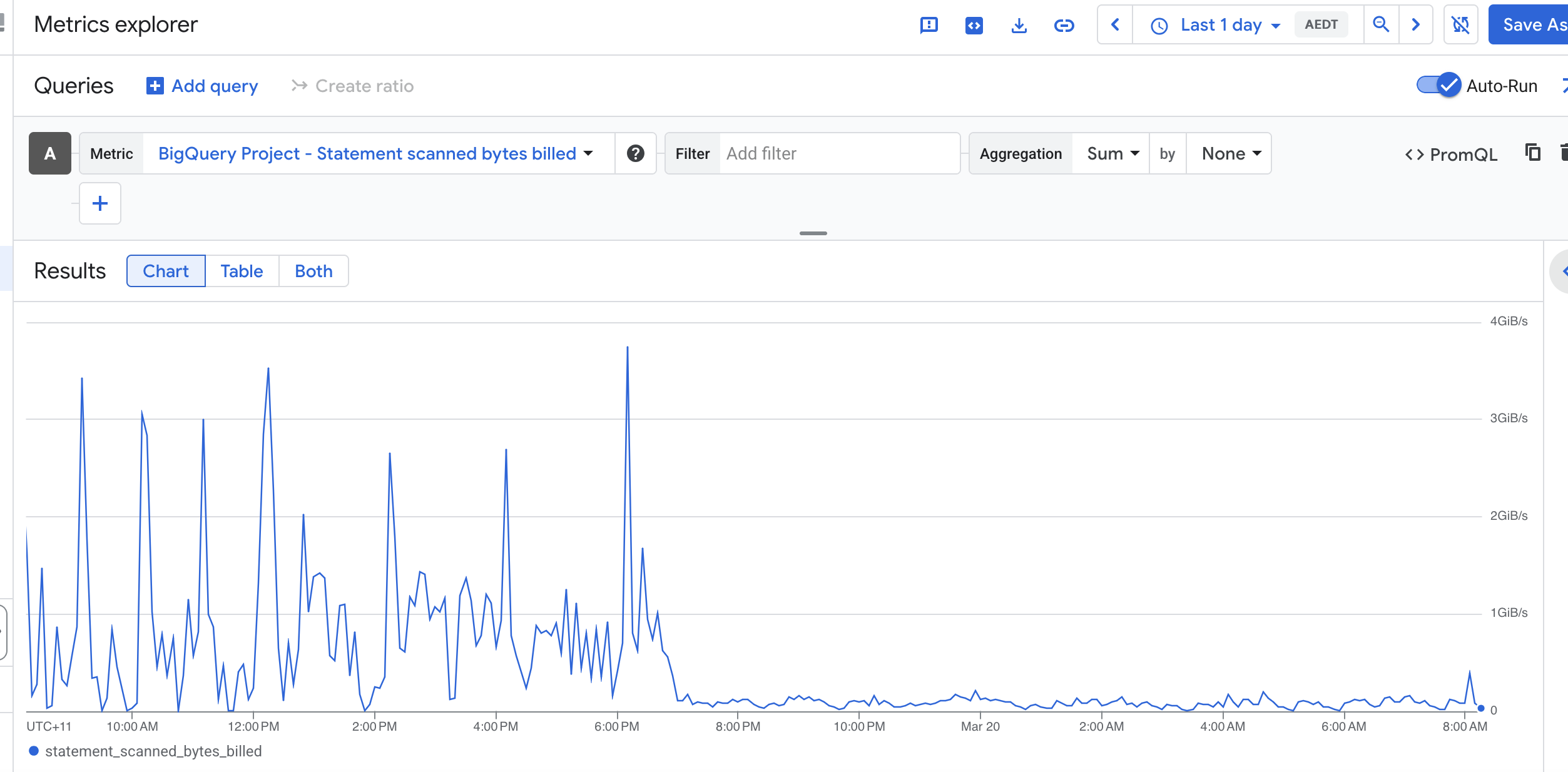
Since ingestion happened in many small batches, the same table was scanned repeatedly, which pushed bytes billed much higher than expected.

The fix was:

stop updating chunk_terms during ingest
write only the primary records during ingestion
move token indexing to a scheduled Cloud Run backfill job
process recent or missing documents in batches
scope each MERGE tightly and dedupe terms before insert

The key lesson is simple: in BigQuery, workload shape matters. A workload made of many tiny MERGEs can cost much more than one built from fewer batched operations, even if the logical output is the same.

To see where BigQuery spend is really going, INFORMATION_SCHEMA.JOBS_BY_PROJECT is extremely useful. These are the first queries I run.

1) Top expensive jobs in the last 7 days

Use this to find the biggest individual jobs by bytes billed.

SELECT
  creation_time,
  job_id,
  user_email,
  statement_type,
  total_bytes_billed,
  total_bytes_processed,
  query
FROM `PROJECT_ID.region-us-central1`.INFORMATION_SCHEMA.JOBS_BY_PROJECT
WHERE creation_time >= TIMESTAMP_SUB(CURRENT_TIMESTAMP(), INTERVAL 7 DAY)
  AND job_type = 'QUERY'
  AND total_bytes_billed IS NOT NULL
ORDER BY total_bytes_billed DESC
LIMIT 50;

2) Bytes billed by statement type

This helps separate spend across SELECT, MERGE, UPDATE, DELETE, and INSERT.

SELECT
  statement_type,
  COUNT(*) AS jobs,
  SUM(total_bytes_billed) AS bytes_billed,
  SUM(total_bytes_processed) AS bytes_processed
FROM `PROJECT_ID.region-us-central1`.INFORMATION_SCHEMA.JOBS_BY_PROJECT
WHERE creation_time >= TIMESTAMP_SUB(CURRENT_TIMESTAMP(), INTERVAL 7 DAY)
  AND job_type = 'QUERY'
GROUP BY statement_type
ORDER BY bytes_billed DESC;

3) Bytes billed by referenced table

This shows which tables are associated with the most billed bytes.

SELECT
  CONCAT(t.project_id, ".", t.dataset_id, ".", t.table_id) AS table_name,
  COUNT(*) AS jobs,
  SUM(j.total_bytes_billed) AS bytes_billed
FROM `PROJECT_ID.region-us-central1`.INFORMATION_SCHEMA.JOBS_BY_PROJECT j,
UNNEST(j.referenced_tables) AS t
WHERE j.creation_time >= TIMESTAMP_SUB(CURRENT_TIMESTAMP(), INTERVAL 7 DAY)
  AND j.job_type = 'QUERY'
  AND t.dataset_id = 'drive_ocr'
GROUP BY table_name
ORDER BY bytes_billed DESC;

4) DML bytes billed by table

This is especially useful if you suspect MERGE or other DML statements are driving cost.

SELECT
  statement_type,
  CONCAT(t.project_id, ".", t.dataset_id, ".", t.table_id) AS table_name,
  COUNT(*) AS jobs,
  SUM(j.total_bytes_billed) AS bytes_billed
FROM `PROJECT_ID.region-us-central1`.INFORMATION_SCHEMA.JOBS_BY_PROJECT j,
UNNEST(j.referenced_tables) AS t
WHERE j.creation_time >= TIMESTAMP_SUB(CURRENT_TIMESTAMP(), INTERVAL 7 DAY)
  AND j.job_type = 'QUERY'
  AND j.statement_type IN ('MERGE', 'UPDATE', 'DELETE', 'INSERT')
  AND t.dataset_id = 'drive_ocr'
GROUP BY statement_type, table_name
ORDER BY bytes_billed DESC;

Closing

If you are investigating BigQuery cost, start by identifying:

which jobs bill the most
which statement types dominate spend
which tables show up most often in expensive queries
whether repeated DML is forcing the same tables to be scanned again and again

In my case, the biggest win came from changing the workload pattern, not from reducing the amount of business data itself.

* * Update the region and dataset to fit your workload

trk7's blog